Let’s Explore And Backtrack

RECURSION

When a function calls itself its called recursion. to understand recursion properly let's take an example -:

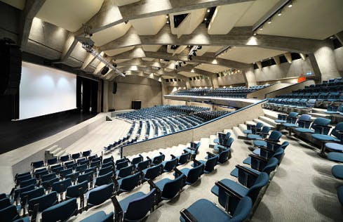
For an inexplicable reason, you want to know the number of rows in your college’s auditorium room. You're too lazy to count so you ask Piyush who is seated in front of you to tell you how many rows are there in front of him. Piyush does the same thing and asks Rithik who is seated in front of him and so on till Prashant who is seated in the first row is asked the question. Prashant can answer Rohit seated in the second row because he can see that there are no more rows in front of him. This is the base case. Rohit adds 1 to Prashant’s answer and tells it to RUHUL who is in the third row and so on until the answer reaches you. Notice that at each step the problem is reduced to a simpler version of the same problem, this is what recursion is - breaking the problem into simpler sub problems.

BACKTRACKING

It is an effective way of solving algorithm problems
Backtracking is an algorithm which is implemented using recursion
It means exploring all the possibilities till we hit a dead end.
A backtracking approach is generally used in the case where there are possibilities of multiple solutions.

let us take a situation to better understand about backtracking

Suppose you are standing in front of three rooms , one of which is having a bag of cash in it , but you don't know which one.

So you'll try all three. First go in the room 1 , if that is not the one , then come out of it , and go into the room 2 , and again if that is not the one , come out of it and go into room 3, so basically in backtracking we attempt solving a sub problem and if we don't reach the position or some case is not satisfied then we backtrack from that position and try to solve via changing the position or the path.

Let us explore one of the example problem of backtracking that can be solved using backtracking to knock down this concept.

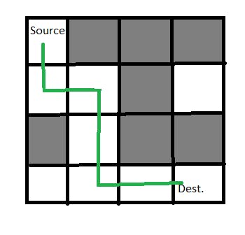
RAT IN THE MAZE

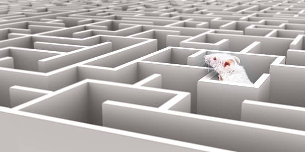
In this we have to explore all the paths and find the solution to reach the end of the matrix.

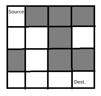
A maze is given as N*N binary matrix of blocks where source block is the uppermost block i.e maze[0][0] and destination block is lower rightmost block i.e maze[N-1][N-1]. In this a rat starts from the source and has to reach the destination. The rat can move in any direction vertically up, vertically down, horizontally right and horizontally left

In the maze matrix, 0 means the block is a dead end and 1 means the block can be used as the path from source to destination.

APPROACH

Form a recursive function, which will follow a path and check if the path reaches the destination or not, If the path does not reach the destination then backtrack and try other paths and if the path reaches the destination then print all the paths.

path to follow.png

SOURCE CODE

def printmazehelper(x, y, maze, n, solution):

    # if we reach the last part of the matrix 
    if x == n-1 and y == n-1:             
        solution[x][y] = 1
        print(solution)
        return

    #base case or the blocking points
    if x < 0 or y < 0 or x >= n or y >= n or solution[x][y] == 1 or maze[x][y] == 0:
        return

    solution[x][y] = 1
    #for moving right , left , down , up
    printmazehelper(x+1, y, maze, n, solution)
    printmazehelper(x, y+1, maze, n, solution)
    printmazehelper(x-1, y, maze, n, solution)
    printmazehelper(x, y-1, maze, n, solution)
    solution[x][y] = 0
    return


def printmaze(maze):
    #to get length of the maze
    n = len(maze)                  
    # initially assigning 0 to solution matrix
    solution=[[0 for j in range(n)] for i in range (n)]        
    printmazehelper(0, 0, maze, n, solution)          

n = int(input())
maze = []
for i in range(n):
    row = [int(ele) for ele in input().split()]
    maze.append(row)
printmaze(maze)

OUTPUT

4
1 1 1 1
1 0 1 1
1 1 0 1
1 1 1 1
[[1, 0, 0, 0], [1, 0, 0, 0], [1, 0, 0, 0], [1, 1, 1, 1]]   # 1st path
[[1, 0, 0, 0], [1, 0, 0, 0], [1, 1, 0, 0], [0, 1, 1, 1]]   # 2nd path
[[1, 1, 1, 0], [0, 0, 1, 1], [0, 0, 0, 1], [0, 0, 0, 1]]   # 3rd path
[[1, 1, 1, 1], [0, 0, 0, 1], [0, 0, 0, 1], [0, 0, 0, 1]]   # 4th path

Process finished with exit code 0

Pros and cons of using Backtracking

Pros :

It is very intuitive to code .
It is a step-by-step representation of a solution to a given problem , which is easy to understand.
It is very easy to implement and contains fewer lines of code, as all backtracking codes are generally few lines of recursive function code.

Cons :

It is very time inefficient , when branching factor is large.
It has large space complexity as we are using recursion.

I hope you enjoyed reading this Blog😊and learned something new from this blog 🎉. You can also connect with me on LinkedIn

Mayank Jha's Blog